
In brief
Each PV area is divided into many calculation points as seen from the observation point. The position of the area in space follows from its outline and heights, the orientation of the modules from tilt, azimuth and, where applicable, cross tilt or tracking. The two inputs are independent of each other and are to be checked separately.
Before reflections are checked, it is established where the module surface lies in space, how its modules are oriented and which part of it is visible from the observation point.
V.2.1 Position and orientation
Two groups of inputs work together:
| Group | Inputs | Determines |
|---|---|---|
| Position | corner points, ground levels (GL), bottom edge and top edge, terrain under the area | where the area lies in space and where calculation points arise |
| Orientation | azimuth, tilt, cross-tilt; for trackers the tracking parameters | the surface normal and thus the reflection direction |
The two groups are independent of each other. The surface normal is not derived from the drawn geometry: an area drawn flat carries exactly the tilt and azimuth entered. A correct outline therefore says nothing about whether the orientation is correct, and vice versa; both must be checked separately (Ch. 7.3, Ch. 7.4).
The normal is built from the upward vertical: the tilt tips it towards the facing direction, the cross-tilt tips it sideways, and the azimuth turns it to the compass direction. All points of an area carry the same normal. For trackers, the normal changes with every time step (section V.2.5).
PV areas with "Dual Orientation" (east-west) are split into two PV areas with the same outline for the calculation: one with the azimuth entered and one turned by 180°; for the second half the cross-tilt is applied with the opposite sign, so that both follow the same mounting structure. Each of the two orientations is thus applied over the entire outline (Ch. 7.3).
V.2.2 Geometry of the PV area
The calculation builds a triangle mesh from each PV area in a local coordinate system (east, north, height above sea level) whose origin lies at the centre of all corner points.
| Installation type | Model |
|---|---|
| Ground-mounted, rack-mounted on a roof | closed body between bottom edge and top edge above the terrain or roof |
| Roof-parallel | one surface through the corner points, without volume |
| Façade (two corner points) | a vertical rectangle between bottom edge and top edge |
| Façade with more than two corner points (e.g. from KML) | one surface through the corner points without volume, as for a roof-parallel system |
Continuous body instead of individual rows. Racked installations are modelled as a continuous body; row gaps are omitted. On open land the body follows the terrain under the area, formed from corner heights and support points (Ch. 7.5).
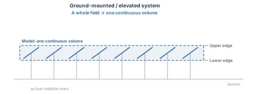
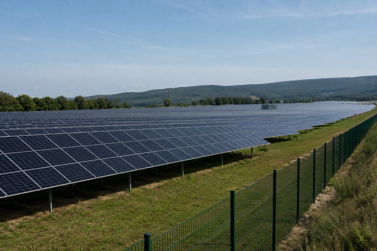
What reflects. The top of the body and its side band from the bottom to the top edge count as module surface; whether the observer sees the front or the back of the modules there is decided by the module normal. The underside of the body and the plinth from the ground to the bottom edge do not reflect, but they occlude what lies behind them. If several parts of the same body lie one behind the other in a viewing direction, the one closest to the observation point applies.
Back side. If the observation point sees a part of the module surface from behind, no reflection arises there. For ground-mounted and racked installations this also applies to a grazing view at more than 89° to the normal, because one actually sees edges and backs of the module rows there; for facades and roof-parallel areas only the view from behind counts. Such parts appear in the report's 3D perspective as non-reflecting surface (Ch. 14).
Excluded areas. Excluded areas are cut out of every overlapping PV area in plan view before the calculation; no calculation points arise there. Façades with two corner points are not cut. If a PV area lies entirely under excluded areas, the simulation stops with a message (Ch. 7.7).
Differentiated cross-tilt. If zones with their own cross-tilt are drawn for an area, the calculation splits the area into sub-areas, each with its own normal. The sub-areas share the point grid of the whole area; where two sub-areas overlap in the same viewing direction, the nearer one applies. In the result, the sub-areas are merged back under the original PV area (Ch. 7.6).
No mutual occlusion. Each PV area is considered on its own. A PV area does not shade another one and does not block its reflection path; this also applies to the two halves of a dual-orientation installation. Such occlusion can be modelled with an obstacle (Ch. 10.1).
V.2.3 Two grids
The calculation works in angles, not in metres: what counts for glare is how large an area appears to the observer. One metre of module edge subtends a little over 1° at 50 m and about 0.1° at 500 m. Both grids of this step are therefore angular grids in azimuth and elevation, measured from the observation point.
Each calculation point is a line of sight. From the observation point, a ray is intersected exactly with the triangle mesh of the area for each direction of the grid; the intersection is the reflecting point. Straight edges of the area appear to the observer as curved arcs, clearly so at close range or a steep view. The grid therefore covers the area up to these curved edges, not only up to the line connecting the corners (since engine version 2026.10.11).
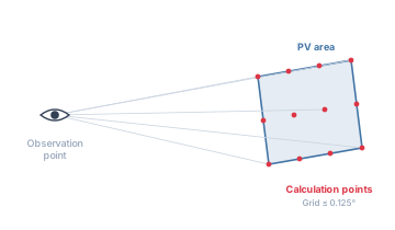
| Grid | Spacing | Task |
|---|---|---|
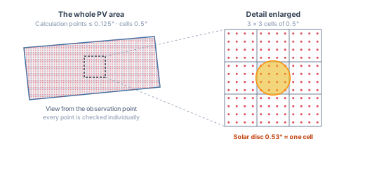
| Cell grid | 0.5° × 0.5°, fixed | assessment unit: for each cell and minute it is decided whether a reflection reaches the observation point |
| Point grid | 0.125° or finer, per PV area and axis | measured values within the cells: solid angle, occlusion, position in the field of view, vertical extent |
The cell grid is the assessment unit. The cells are anchored at 0°; their centres lie on multiples of 0.5°. The hit check, glare minutes, filters, heatmaps and the Excel detail data all refer to these cells. The cell size follows the physics of glare, not the size of the installation: the sun subtends about 0.53°, its mirror image cannot be smaller than about one cell, and the lobes of real modules are several degrees wide. The fixed value also keeps the glare minutes of different projects comparable.
The point grid supplies the measured values. The step size is chosen per PV area and separately for width and height: so that about 40 points fit across the visible extent of the area, at least 30, but no coarser than 0.125°. The step size is snapped to an integer fraction of 0.125° (0.125°/n), so that the points fill each cell without remainder. Separate axes are needed because distant areas appear foreshortened: a ground-mounted installation 7 km away can appear 0.24° wide but only 0.005° high. The smallest and largest step sizes used are listed in the report under "Spatial resolution". Per area and observation point, a maximum of 20,000 points applies; it takes precedence over the target of at least 30 points but never coarsens the grid beyond 0.125°. At the edge of the area, a calculation point carries the share of its grid cell that lies on the module surface, determined with 4 × 4 sub-points; if the centre of such an edge cell lies beside the area, a point on the module part of the cell represents it.
A third grid concerns only the display. For the 3D perspective and the reflection map, the 0.5° cells are additionally subdivided into cells of 0.25° or 0.125°, as fine as the point grid fills them, limited by a maximum number of cells per area and observation point. For the module type "Perfect mirror" and for areas with differentiated cross tilt, they stay at 0.5°. This subdivision distributes the solid angle of a 0.5° cell over its sub-cells; glare minutes and filter decisions remain at 0.5°.
Deep dive: accuracy of the hit check
The hit check compares the cell centres with the lobe. So that no cell is missed whose edge still reaches into the lobe, the lobe is widened by half the cell diagonal (0.354°). The whole cell then counts as hit. For the glare minutes this widening works in the direction of more glare; for lobes several degrees wide it amounts to a few percent. A visible calculation point of a cell at the lobe edge contributes to the solid angle only with the share of its area that lies in the lobe; a cell entirely within the lobe counts in full.
For narrow lobes, the widening would be of the order of the lobe itself. If the smallest semi-axis of the lobe (including the solar radius) is smaller than 1.5° and the largest smaller than 6°, the check is therefore carried out point by point on the point grid. Solid angle and vertical extent then arise only from the points actually hit, the solid angle at the lobe edge again with the area share inside the lobe; the widening is half the diagonal of the point grid, about 0.09° at 0.125°. The decision is made per time step, because the same lobe can be narrow at steep incidence and wide at shallow incidence. The perfect mirror is always checked point by point.
Deep dive: orders of magnitude and decision rules per cell
Grid spacings in reality, perpendicular to the line of sight:
| Distance to the PV area | Spacing of calculation points at 0.125° | Edge length of a cell (0.5°) |
|---|---|---|
| 50 m | approx. 11 cm | approx. 44 cm |
| 100 m | approx. 22 cm | approx. 87 cm |
| 250 m | approx. 55 cm | approx. 2.2 m |
| 500 m | approx. 1.1 m | approx. 4.4 m |
If the calculation points of a cell give different results, the cell decides per attribute as follows:
| Attribute | The cell counts as … | if |
|---|---|---|
| blocked by obstacle or terrain | blocked | more than half of its points are blocked; at exactly half it remains visible |
| outside the field of view | outside | all its points lie outside |
| shaded | shaded | the ray from the centroid of its points towards the sun hits an obstacle, the sun is below the horizon line or (with terrain occlusion) not above the terrain at the nearest sampling point |
For a visible cell, solid angle and vertical extent count only from its unblocked points. A predominantly blocked cell carries the full value, so that it shows its unblocked effect when the filter "Reflection blocked by obstacle" is switched off (Ch. V.8).
V.2.4 Cross-tilt
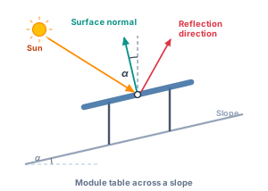
If a module table stands across a slope, the module row tilts sideways relative to the main tilt. The surface normal turns to the side, the effective azimuth and effective tilt shift, and with them the reflection direction. Even 1° to 2° of cross-tilt noticeably shift the glare-affected area sideways over larger distances. PV areas with markedly different cross-tilt can be represented as separate PV areas or with the differentiated cross-tilt using zones (Ch. 7.6).
V.2.5 Tracked systems
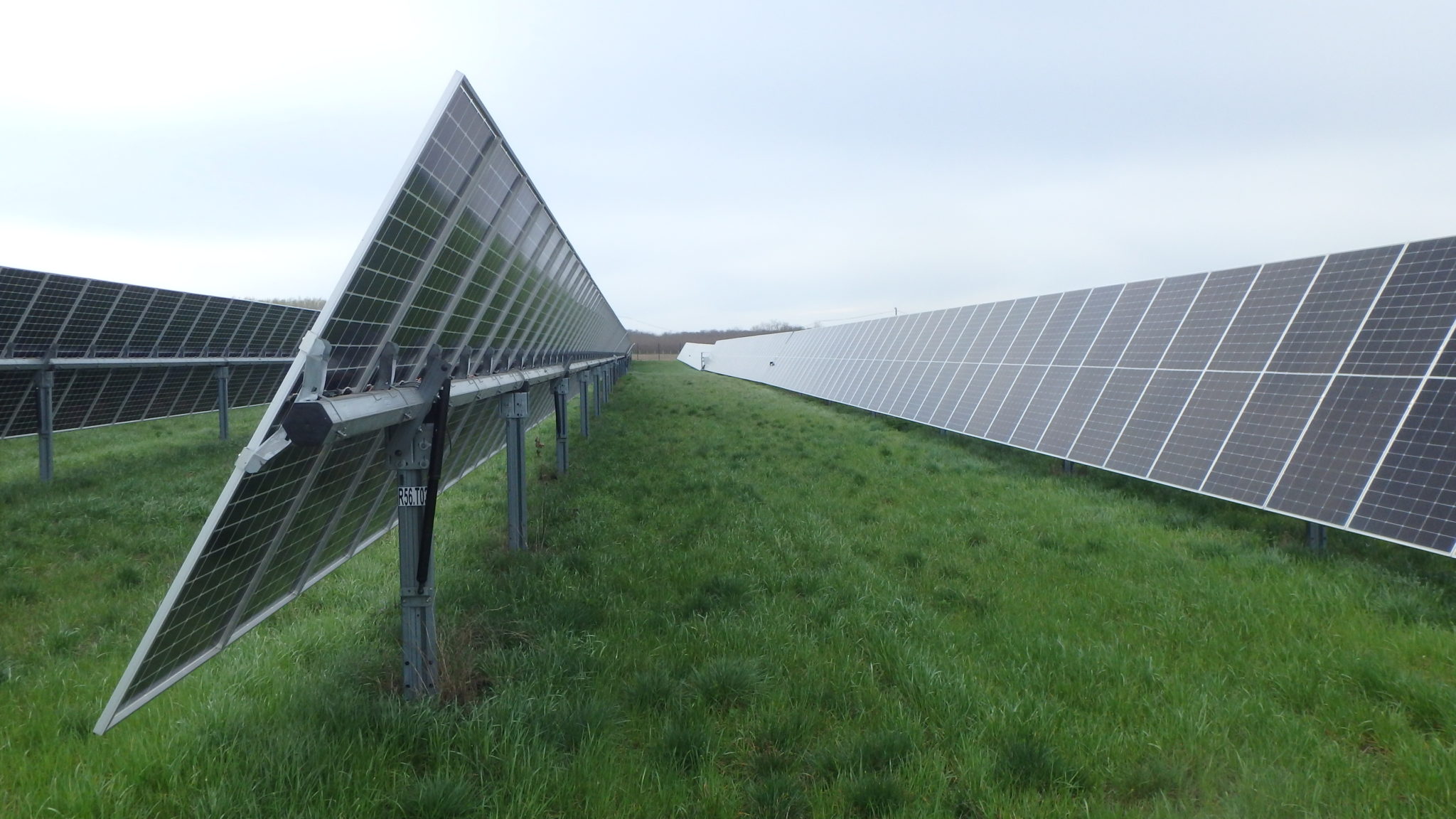
For single-axis tracked systems (trackers), the orientation changes over the day. The calculation determines the tracking angle for every time step from the solar position and from that the surface normal; the rest of the chain (V.3 to V.7) runs unchanged. The twelve monthly curves in the editor and the report (each on the 21st of a month) come from the same function and serve as illustration; they do not enter the calculation.
Deep dive: tracking angle and rotation
- Tracking angle. Per time step with the pvlib function for single-axis tracking, from the apparent solar zenith angle and solar azimuth, "Axis Orientation", "Axis Tilt" and "Module Angle Range" (largest rotation angle ±). The basis is the tracking geometry according to Lorenzo et al. (2011) and Marion and Dobos (2013).
- Backtracking. If "Backtracking" is active, the function rotates the modules back at low sun so that the rows do not shade each other at the Ground Coverage Ratio (GCR) entered. The terrain across the axis is assumed to be level; slope-aware backtracking according to Anderson and Mikofski (2020) is not applied.
- Rest angle. While backtracking reduces the angle, its magnitude does not fall below the "Rest Angle" (Stow angle); it has no effect at midday.
- Axis tilt. A positive axis tilt means that the axis descends towards the axis orientation entered.
- Missing values. Axis orientation, axis tilt, angle range and backtracking are required, and with backtracking switched on so are GCR and rest angle. If one is missing, the simulation does not start; the to-do list names the field (Ch. 7.3). The calculation does not insert substitute values.
- Night. When the sun is below the horizon, there is no tracking angle and no hit.
- Rotation. The normal results from rotation about the axis (Rodrigues' formula); positive angles tip it towards the side of axis orientation + 90°. No cross-tilt is applied to trackers.
- Back side. For trackers, the check for back side and grazing view (Ch. V.3) runs per time step with the normal of that time step. In the point-by-point check it applies to every hit calculation point. On the cell grid the cell centre decides; if the boundary runs through the cell, its calculation points decide: the cell remains as soon as one of them is in front, and carries only the solid angle of the points in front.